
|
The Atlantic Coastal Plain Province encompasses the easternmost part of Virginia (fig. 1), an area of approximately 13,000 mi2. The Coastal Plain in Virginia is underlain by eastward dipping strata of unconsolidated to partly consolidated sediments of Cretaceous, Tertiary, and Quaternary age that unconformably overlie bedrock of the Piedmont Province (fig. 2). The boundary between the Coastal Plain sediments and Piedmont is termed the "Fall Line".
A hydrogeologic framework of the Virginia Coastal Plain was developed as part of the Regional Aquifer System Analysis (RASA) program of the U.S. Geological Survey (USGS) (Meng and Harsh, 1988). Ground water in the Coastal Plain is present primarily in pores in the sediments. Thick sequences of porous and permeable strata form regional aquifers, and less permeable strata form confining units between the aquifers. The Columbia aquifer is unconfined throughout the Virginia Coastal Plain. It is regionally extensive in the eastern part of the area but is restricted to the floodplains and terraces of major rivers in the western part. The Yorktown-Eastover aquifer is confined beneath the Columbia aquifer in the eastern part of the area; the aquifer is unconfined in the western part where it crops out along uplands that separate the major rivers. All the other aquifers generally are confined throughout the area, except small parts of some aquifers that crop out near the Fall Line.
Ground water in the Virginia Coastal Plain is recharged principally by infiltration of precipitation and percolation to the water table. Most of the unconfined ground water flows relatively short distances and discharges to nearby streams, but a small amount flows downward to recharge the deeper, confined aquifers (fig. 2). Flow through the confined aquifers primarily is lateral in the down-dip direction to the east and toward large withdrawal centers and major discharge areas near large rivers and the Atlantic coast. Dense saline water at the interface between freshwater and saltwater causes the confined ground water to discharge by upward flow across intervening confining units.
Several studies have analyzed ground-water flow in the Virginia Coastal Plain. During the early 1980's, a digital numerical model (fig. 3) was constructed as part of the RASA program, to analyze the entire ground-water-flow system in the Virginia Coastal Plain (Harsh and Laczniak, 1990). During the late 1980's, the USGS conducted more detailed studies of smaller areas within the Virginia Coastal Plain, including southeastern Virginia (Hamilton and Larson, 1988) and the York-James Peninsula (Laczniak and Meng, 1988). During the early 1990's, the RASA regional-scale model was revised by the USGS, in cooperation with State and local agencies, to incorporate reinterpretations of the hydrogeologic framework from the southeastern Virginia and York-James studies. Because the revisions were based on earlier documented studies, the regional-scale model was not recalibrated and the revised form of the model was not published at that time. Concurrently, a geographic information system (GIS) was integrated with the model (Focazio and Samsel, 1993) to provide a means to efficiently procesys and use model input and output data.
Aquifers in the Virginia Coastal Plain are a heavily used water resource. The rate of ground-water withdrawal is estimated to have been close to zero during the late 1800's, but has increased nearly continuously during the 20th century (Harsh and Laczniak, 1990). During 1992, a withdrawal rate of approximately 94 Mgal/d from Coastal Plain aquifers was reported by major ground-water users to the Virginia Department of Environmental Quality (DEQ) (Hammond and Focazio, 1995). Ground-water levels have declined as a result of the large withdrawals and, by 1993, were as deep as 160 ft below sea level in observation wells near major pumping centers (Hammond and others, 1994a, 1994b, 1994c).
Both the original model (Harsh and Laczniak, 1990) and the revised model have been used to address the need for management of the ground-water resource. DEQ has based ground-water regulatory actions partly on simulation results of both models, and has accepted use of the revised model as a means to evaluate the potential effects of proposed withdrawals. The revised form of the model currently (1998) in use, however, has not been documented. In addition, the USGS has performed model simulations as part of its ongoing studies in cooperation with DEQ. Major ground-water users report withdrawals annually to DEQ to satisfy regulatory requirements. Regional water-level declines have been estimated on the basis of periodically updated ground-water-withdrawal data. Simulations of the water-level declines have been performed on the basis of withdrawals reported from 1982 through 1994, but the simulation results have not been published.
Revisions to the regional ground-water-flow model of the Virginia Coastal Plain are documented in this report. The overall design of the model is described, but details of model specifications, mathematical basis, design rationale, and calibration and sensitivity analyses are specifically excluded. Earlier documented studies are referenced extensively for supportive information.
Model revisions made during 1990-94 by personnel of the USGS Virginia District Office are presented. Changes to model-input data that numerically represent the hydrogeologic framework are summarized and described. Model-layer aquifer assignments and representation of the unconfined aquifer are discussed. The values of transmissivity and vertical leakance assigned to the various model layers are presented and compared to those for the original model and to the values used in subsequent modeling studies. Possible effects of the revisions are illustrated by a simulation performed using the revised model and the well withdrawal rates specified in the original model for the period 1978-80.
Considerations for continued use of the model are discussed, and the potential support of resource-management efforts provided by the model is described. Design features of the model that limit its accuracy and constrain its application are explained, and the capabilities of the model needed to maintain its usefulness are discussed.
The author wishes to thank Terry Wagner, Mary Ann Massie, and T. Scott Bruce, of the Virginia Department of Environmental Quality, for program and planning support. Michael J. Focazio, of the U.S. Geological Survey, provided much of the information on the design of, and revisions made to, the model. Thanks are also extended to numerous drillers and owners of water-supply wells for providing well-construction data and water-level data. The U.S. Environmental Protection Agency provided funding to the Virginia Department of Environmental Quality for modeling activities in support of ground-water resource management.
Ground-water flow in the Virginia Coastal Plain has been simulated using the quasi-three-dimensional approach described by Bredehoeft and Pinder (1970). The original regional model (Harsh and Laczniak, 1990) was based on the finite-difference-model program code of Trescott (1975) as modified by Leahy (1982). Subsequent studies in southeastern Virginia (Hamilton and Larson, 1988) and in the York-James Peninsula (Laczniak and Meng, 1988) were based on the modular finite-difference-model program code of McDonald and Harbaugh (1984). The revised regional model is based on the updated modular model code (McDonald and Harbaugh, 1988), popularly known as MODFLOW.
In all of the above studies, aquifers are represented by model layers that are (1) arranged vertically, (2) specified as being under either confined or unconfined conditions, and (3) discretized laterally by a block-centered grid. Aquifer transmissivities, storage coefficients, and initial water levels are specified for each grid cell within each layer. Confining units between aquifers are not included as separate layers. Instead, vertical leakance values are specified for the cells in each aquifer layer to represent hydraulic connections between adjacent layers. Hence, horizontal flow through the aquifers is represented by flow within each layer, and vertical flow between aquifers is represented by flow between adjacent layers. In addition, boundary conditions of head and (or) flow are specified along the margins of each layer, and any hydraulic stresses (sources of recharge or discharge) are specified for the cells in which they are located.
Simulation is performed by executing the model program. The input data described above are "read" by the program, and systems of partial differential equations that approximately represent ground-water flow in three dimensions are iteratively solved to calculate values of hydraulic head and flow rate for each cell. A simulation is specified as being either (1) steady state, in which one set of stresses is imposed independently of time, and changes in storage are not considered; or (2) transient, in which stresses can be changed over time, and water can be placed into or removed from storage.
Many design features are shared between the original (Harsh and Laczniak, 1990) and revised ground-water-flow models of the Virginia Coastal Plain. The areas of both models are delineated by a grid that spans an area of approximately 17,000 mi2 of uniformly spaced square cells scaled to 3.5 mi on each side (fig. 3). The model area encompasses the entire Coastal Plain in Virginia and extends eastward from the Fall Line to beyond the Atlantic coast, southward to the Albemarle Sound in North Carolina, and northward across the Potomac River and into Maryland.
Both models include 10 layers (table 1), representing the regional aquifers (fig. 2) that were delineated as part of a hydrogeologic framework of the Virginia Coastal Plain (Meng and Harsh, 1988). None of the aquifers span the entire area of the model grid. The model grid was extended offshore beyond the margins of all of the aquifers (fig. 3) to facilitate incorporation of the original model into a larger model of the entire northern Atlantic Coastal Plain (Leahy and Martin, 1993). The aquifers are bounded laterally where the sedimentary strata that comprise them either (1) pinch out westward toward the Fall Line, or (2) become increasingly fine-grained eastward or reach a water-density barrier along the saltwater interface toward the coast. Accordingly, the western aquifer margins corresponding to the Fall Line, and the eastern margins corresponding to fine-grained sediments or to the saltwater interface, are specified in the model layers as no-flow boundaries. As a result, the positions of the aquifer margins vary widely among the aquifers, and the areal distribution of the aquifers has a complex overlapping configuration. In order to represent parts of the model area in which one or more aquifers are absent, corresponding model layers are assigned zero transmissivities and non-zero vertical leakances, so that only vertical flow between the adjacent layers is allowed (Harsh and Laczniak, 1990) (see section "Transmissivity and Vertical Leakance Values").The aquifers are not bounded laterally to the north or south but extend from Virginia into adjacent States. Accordingly, aquifer margins along the northern and southern sides of the model grid are specified in the model layers as lateral-flow boundaries. Flow to or from model cells is held constant at specified rates that represent flow to or from parts of the aquifers that extend beyond the model grid. Flow values assigned to the cells along the northern and southern sides of the grid were calculated by a larger model of the northern Atlantic Coastal Plain (Harsh and Laczniak, 1990).
Table 1. Aquifer and confining unit numbers and designations for layers of the original and revised ground-water-flow models of the Virginia Coastal Plain |
|||
|---|---|---|---|
Original model |
Revised model |
||
Layer No. |
Designation |
Layer No. |
Designation |
| none | surface water | none | removed |
| 10 | Columbia aquifer; Yorktown confining unit | 1 | Columbia aquifer; Yorktown confining unit |
| 9 | Yorktown-Eastover aquifer; Saint Marys confining unit | 2 | Yorktown-Eastover aquifer; Saint Marys confining unit |
| 8 | Saint Marys-Choptank aquifer; Calvert confining unit | 3 | Saint Marys-Choptank aquifer; Calvert confining unit |
| 7 | Chickahominy-Piney Point aquifer; Nanjemoy-Marlboro confining unit | 4 | Chickahominy-Piney Point aquifer; Nanjemoy-Marlboro confining unit |
| 6 | Aquia aquifer; Confining unit 5 | 5 | Aquia aquifer; Peedee confining unit |
| 5 | Aquifer 5; Confining unit 4 | 6 | Peedee aquifer; Virginia Beach confining unit |
| 4 | Aquifer 4; Brightseat-upper Potomac confining unit | 7 | Virginia Beach aquifer; Brightseat-upper Potomac; confining unit |
| 3 | Brightseat-upper Potomac aquifer; middle Potomac confining unit | 8 | Brightseat-upper Potomac aquifer; middle Potomac confining unit |
| 2 | middle Potomac aquifer; lower Potomac confining unit | 9 | middle Potomac aquifer; lower Potomac confining unit |
| 1 | lower Potomac aquifer | 10 | lower Potomac aquifer |
Vertical model boundaries in the original regional model included an extra layer to represent surface water (in addition to the aquifer layers), thereby simulating streambed leakage to or from the underlying unconfined aquifer layer. The surface-water layer is removed from the revised model (see section "Layers and Boundary Conditions"). The lowermost layer of both the original and revised models is bounded across its base by a no-flow boundary that represents the underlying bedrock.
Areal recharge to the unconfined aquifer layer was specified in the original regional model at a rate of 15 in/yr, but is removed from the revised model. Instead, constant-head values are assigned to represent the water table (see section "Layers and Boundary Conditions").
Ground-water-withdrawal rates are specified for model cells in which pumping wells are located. The withdrawal rates for individual wells located within a single cell and layer are summed to represent the withdrawal rate for the entire cell. In order to determine the effects of increasing withdrawals from 1890 through 1980, transient simulations were performed by using the original model, in which 10 stress periods were specified to discretize the period (Harsh and Laczniak, 1990). By contrast, only steady-state simulations have been performed using the revised model (see section "Changes to Model-Input Data").
Computer files that contain the model design information constitute the input data for the revised model. The files are read during execution of the model program, which creates additional files that contain simulated water levels and flow rates and that constitute the output data. The input files, output files, and program code comprise the actual model, which is separate and distinct from a geographic information system (GIS) that was developed to represent the model framework (Focazio and Samsel, 1993).
The GIS contains some of the same data used in the revised model, and was developed by Focazio and Samsel (1993) using the ARC/INFO system to facilitate revision of the model and to display model and related data. A GIS is an integrated computer system of datasets and programs used to collect, manage, analyze, and display spatially referenced data. Model simulation uses the model-program code and input and output files described above, and does not involve or depend on the GIS.
In ARC/INFO, similar types of information on a given area are stored in individual datasets called coverages. A polygon coverage was constructed to correspond to the regional model grid. Individual polygons in the coverage represent grid cells. Data stored in the coverage under each polygon correspond in part to data assigned to the grid cells in the actual model. In addition, the polygon coverage includes ancillary hydrogeologic information that is not used by the model, such as aquifer and confining unit elevations and thicknesses, and provides a means to examine and analyze different aspects of the hydrogeologic framework. Thus, the polygon coverage is separate from, but related to, the input and output files of the actual model, and contains a broader array of information. Separate coverages containing subsets of the same information also were created (Focazio and Samsel, 1993).
Input files that constitute the revised model are available from the USGS Virginia District Office. Revisions to the model are summarized and described below. Specific changes to data contained in the input files are not described in detail. Documentation of the MODFLOW program (McDonald and Harbaugh, 1988) explains the content and organization of the input files.
The model was revised based generally on the following procedure (M.J. Focazio, U.S. Geological Survey, oral commun., 1997). First, a reevaluation was made of the original hydrogeologic framework (Meng and Harsh, 1988) along with the hydrogeologic frameworks delineated by the two subsequent studies in southeastern Virginia (Hamilton and Larson, 1988) and the York-James Peninsula (Laczniak and Meng, 1988). The frameworks of the subsequent studies, however, were not used simply to replace the corresponding parts of the original framework. Instead, hydrostratigraphic interpretations of geophysical well logs that are documented for all three studies were revised and integrated to redelineate the geometry (elevation, thickness, and lateral extent) of the aquifers and confining units. Because three separate sources of information were used, in some areas the revised framework is not identical to any one of the earlier frameworks.
GIS data-processing capabilities were then employed to generate revised model-input data based on the revised hydrogeologic framework. Because the original and revised models are based on the same model grid (fig. 3), transmissivity and vertical leakance values from the original model were assigned directly to model layers for parts of aquifers and confining units where their geometry remained unaltered. For those parts of aquifers and confining units for which the geometry was modified, new values of transmissivity and vertical leakance were calculated. Because the model grid for the original and revised model differs from those constructed for the subsequent studies (southeast Virginia and the York-James Peninsula), values of transmissivity and vertical leakance from the subsequent studies were averaged during calculation of the revised values.
Whereas the original model performed simulations under transient conditions, the revised model was specified to perform simulations under steady-state conditions. Under transient conditions, flow rates into and out of the model are varied among different specified time increments, called pumping periods. Additional water is internally supplied and removed during the same pumping periods as flow into and out of storage. Volumes of water entering and leaving the model are calculated as the products of the flow rates and the durations of the pumping periods. A set of simulated water levels is produced for each pumping period, and changes in simulated water levels between pumping periods represent changes in water level in response to changes in flow rates. By contrast, under steady-state conditions, simulated water levels are recalculated by iterative solutions of the ground-water-flow equations until the flow system reaches an equilibrium condition and simulated water levels no longer change significantly in further iterations. A water-level change criterion of 0.001 ft is specified in the revised model for iteration to cease. Only one set of simulated water levels is produced as model output, which represents an equilibrium between rates of flow into and out of the model in which storage does not change.
Projected use of the revised model was not expected to require transient simulation. Sensitivity analyses of the transient simulations performed using the original model indicated that the flow system was near equilibrium by the end of each pumping period (Harsh and Laczniak, 1990). Therefore, any differences in simulated water levels between the original model and the revised model that could result from differences between transient and steady-state conditions would probably be small.
A numbering scheme is needed to designate and refer to model layers and to assign the aquifers to their respective layers. In the original framework (Meng and Harsh, 1988), the original model (Harsh and Laczniak, 1990), and the GIS (Focazio and Samsel, 1993), model layers were numbered starting with layer 1 at the bottom to designate the lowermost aquifer and proceding upward (table 1). The revised model, however, is based on the MODFLOW program code in which numbering proceeds in the opposite order--from top to bottom (table 1). Accordingly, the model-layer numbering used for this report follows the order of the model-input data specified for the MODFLOW program, and proceeds from layer 1 at the top to layer 10 at the bottom.
Aquifer designations and their correspondence to geologic formations are documented fully for the original framework (Meng and Harsh, 1988) and the original model (Harsh and Laczniak, 1990), and they are not reiterated here. Other than the reversed numbering, most of the designations have been retained in the revised model (table 1). Two layers have been redesignated in the revised model to represent different aquifers than in the original model, largely on the basis of the subsequent study in southeastern Virginia (Hamilton and Larson, 1988). Both aquifers occupy only small parts of the model area and are present mostly in North Carolina. Layer 5 in the original model included both the Peedee Formation in North Carolina and the Severn Formation in Maryland, but the corresponding layer in the revised model (layer 6) includes only the Peedee Formation and is referred to as the Peedee aquifer. Layer 4 in the original model included the Black Creek Formation and Middendorf Formation, both in North Carolina, but the corresponding layer in the revised model (layer 7) has been redesignated as the Virginia Beach aquifer, which extends northward into southeastern Virginia.
The no-flow model-layer boundaries (Fall Line, fine-grained sediments, saltwater interface, and basement rock) were changed slightly from the original model to reflect revised lateral extents of the aquifers. For the lateral-flow boundary along the northern and southern sides of the model grid, the revised model uses the most recent (1978-80) flow rates used in the original model (see section "Effects on Simulated Water Levels").
Representation of the unconfined aquifer has been modified in the revised model. During construction of the original model, two conceptualizations were used to simulate the unconfined aquifer. In the first conceptualization, the surface-water layer was not included. Instead, the unconfined aquifer was defined by a constant-head boundary. Model cells were assigned water-table elevations approximately equal to land surface, for layers that represent the aquifer in which the water table is present. In offshore areas, the freshwater equivalent elevation of the coastal water surface was specified. During simulation, the water table was held fixed while flow to or from the cells was allowed to vary. The first conceptualization was used to calculate vertical leakage to and from the confined aquifers. During the second conceptualization, the surface-water layer and recharge to the water table were added, and representation of the unconfined aquifer was changed to allow the water table to fluctuate. The second conceptualization allowed simulations to include lateral flow within the uppermost aquifer, and upward and downward flow to or from surface water.
Projected use of the revised model was not expected to require simulation of lateral flow within the unconfined aquifer, or upward and downward flow to or from surface water. Accordingly, representation of the unconfined aquifer in the revised model was reverted to the first conceptualization used in the original model. The surface-water layer in the original model has been removed (table 1), and recharge to the unconfined aquifer is no longer applied. Constant-head cells are assigned (1) throughout layer 1, which represents the Columbia aquifer and is unconfined across its entire extent; (2) in the western part of layer 2, which represents the Yorktown-Eastover aquifer and is unconfined in outcrop areas along uplands separating the major rivers; and (3) in small parts of some other layers, which represent aquifers that crop out near the Fall Line. The upper vertical boundary that is imposed by the constant-head unconfined aquifer layers on underlying layers in the revised model is hydraulically equivalent to the original model. The primary result of the modification is that flows to and from surface water are no longer represented.
Aquifers are represented in the model by transmissivity values assigned to cells in their corresponding layers. Because the revised model performs steady-state simulations (see section "Effects on Simulated Water Levels"), storage coefficients are not assigned. Transmissivity values control horizontal flow within the model layers. The distributions of transmissivity values in the layers of the revised model are represented by maps (figs. 4-13, at back of report). Those parts of the model layers with transmissivity values greater than zero represent the lateral extents of the aquifers, as indicated by the maps.
Aquifer transmissivities and lateral extents represented by the layers in the revised model appear similar to those of the original model (Harsh and Laczniak, 1990, figs. 13-21) for some layers but dissimilar for other layers. Revised transmissivities of the Columbia, Yorktown-Eastover, and Saint Marys-Choptank aquifers (figs. 4-6) generally are similar to those in the original model, except for the far southwestern part of the Yorktown-Eastover aquifer, where the revised transmissivity values are higher than the original values. In addition, the western margins of the Columbia and Yorktown-Eastover aquifers have been modified, and the southern part of the Saint Marys-Choptank aquifer has been removed. Revised transmissivities of the Chickahominy-Piney Point aquifer (fig. 7) and of the Aquia aquifer (fig. 8) are approximately half of those in the original model. In addition, the eastern margin of the Chickahominy-Piney Point aquifer has been extended seaward, whereas the eastern margin of the Aquia aquifer has been moved landward. Transmissivity values of the layer corresponding to the Peedee aquifer (fig. 9) is not illustrated for the original model and cannot be compared. The revised transmissivity of the Virginia Beach aquifer (fig. 10) spans a similar range of values as the corresponding layer in the original model (aquifer 4), but it has a different areal distribution. In addition, the margins have been extended northward and westward. The revised transmissivity of the Brightseat-upper Potomac aquifer (fig. 11) is approximately twice that in the original model. The margins generally are similar to the original model. Revised transmissivities of the middle Potomac aquifer (fig. 12) and of the lower Potomac aquifer (fig. 13) generally are similar to those in the original model, except for the far northern part of the middle Potomac aquifer, which has a higher revised transmissivity. The margins generally are similar to those in the original model, except that the lower Potomac aquifer has been extended southwestward into North Carolina.
Representation of confining units in both the original and revised models is limited. Confining units are not represented explicitly by separate model layers, but their effect is represented by vertical leakance values specified for aquifer layers that control vertical flow between adjacent layers. Model-input data are organized such that the vertical leakance values assigned to an aquifer layer control vertical flow to or from the adjacent underlying layer and, hence, correspond to the confining unit underlying the aquifer (table 1).
Vertical leakance values do not represent specific confining units in large parts of some layers in either the original or the revised models. The vertical leakance values for a model layer only represent the actual vertical leakances of a specific confining unit in those parts of the model area in which aquifers are present immediately above and below the confining unit. In areas where some aquifers are thin or absent, two or more confining units are in proximity or direct contact, and the vertical leakance values of the corresponding model layers have been adjusted to account for the missing aquifers (Harsh and Laczniak, 1990). In these areas, the vertical leakance values of adjacent layers collectively represent the total vertical leakance of the entire sequence of contiguous confining units, and vertical leakance values of individual model layers do not represent specific confining units. Conversely, in areas where a confining unit is thin or absent, two aquifers are in proximity or direct contact, and the vertical leakance values of the corresponding model layer has been adjusted to account for the missing confining unit and represent the vertical leakance between the contiguous aquifers.
The distributions of vertical leakance values of layers in the revised model are represented by maps (figs. 14-22, at back of report) (fig. 14), (fig. 15), (fig. 16), (fig. 17), (fig. 18), (fig.19), (fig. 20), (fig. 21), (fig. 22). Parts of the model layers are designated in which aquifers adjoining each confining unit are missing and vertical leakance values are not representative of the actual vertical leakances of specific confining units.
Comparisons of revised vertical leakance values to those in the original model are limited. The actual vertical leakances and lateral extents of the confining units are illustrated for the original model (Harsh and Laczniak, 1990, figs. 23-30), with areas shaded to indicate adjustment of the vertical leakance values of model layers to account for missing aquifers. Consequently, only generalized comparisons to the vertical leakances of confining units in the revised model are possible.
Considering only those parts of model layers in which vertical leakance values are representative of the actual vertical leakances of specific confining units (aquifers are present immediately above and below the confining unit), confining unit vertical leakances represented by the layers in the revised model appear similar to those of the original model (Harsh and Laczniak, 1990, figs. 23-30) for some layers but dissimilar for other layers. Revised vertical leakances generally are higher than those in the original model by a factor of about 2-3 in the Yorktown, Saint Marys, Nanjemoy-Marlboro, and middle Potomac confining units. Revised vertical leakances generally are similar to those in the original model for the Calvert, Virginia Beach, and lower Potomac confining units. Revised vertical leakances generally are lower than those in the original model for the Brightseat-upper Potomac confining unit by about one order of magnitude.
In order to evaluate possible effects of revisions to the model, a simulation was performed using the revised model and the well withdrawal rates specified in the original model for the period 1978-80. The total rate of withdrawal is approximately 105 Mgal/d, more than 80 percent of which is from the lower Potomac, middle Potomac, and Brightseat-upper Potomac aquifers.
The distributions of simulated water levels produced by the revised model are represented by maps (figs. 23-32, at back of report), and were compared to those produced by the original regional model using the same withdrawal data (Harsh and Laczniak, 1990, figs. 50-57). Simulations performed by the revised model are specified to be under steady-state conditions, in which one set of stresses is imposed independently of time, and any changes in storage are not considered. Accordingly, only one set of ground-water-withdrawal rates are specified for model cells in which pumping wells are located. In addition, the 1978-80 flow values used in the original model for the lateral-flow cells along the northern and southern sides of the model grid are specified in the revised model (see section "Model Design").
Within the revised lateral extents of the model layers, simulated water levels from the revised model appear similar to those from the original model (Harsh and Laczniak, 1990, figs. 50-57) for some layers but dissimilar for other layers. Simulated water levels in the Columbia aquifer are not illustrated for the original model and cannot be compared. In the revised model, simulated water levels in the Columbia aquifer (fig. 23) primarily represent the water table, and are input to the model as initial water levels assigned to constant-head cells (see section "Layers and Boundary Conditions"). Simulated water levels in the Yorktown-Eastover aquifer (fig. 24) and in the Saint Marys-Choptank aquifer (fig. 25) generally are similar to the original model. Simulated water levels in the Chickahominy-Piney Point aquifer (fig. 26) and in the Aquia aquifer (fig. 27) generally are similar to the original model in the southern and far western parts of the aquifers, but are higher in the central and northern parts by about 20 ft. Simulated water levels in the Peedee aquifer (fig. 28) are not illustrated for the original model and cannot be compared. Simulated water levels in the Virginia Beach aquifer (fig. 29) generally are similar to the corresponding layer in the original model (aquifer 4). Simulated water levels in the Brightseat-upper Potomac aquifer (fig. 30) generally are similar to the original model in the northern and northeastern parts of the aquifer, but are lower in the southern and far western parts by about 30 ft, and are higher near the center of the aquifer by about 30 ft. Simulated water levels in the middle Potomac aquifer (fig. 31) generally are similar to those in the original model in the southern and far western parts of the aquifer, but are higher in the northern and central parts by about 20 ft, and are lower in the far southeastern part by about 20 ft. Simulated water levels in the lower Potomac aquifer (fig. 32) generally are similar to those in the original model in the central and southern parts of the aquifer, but are higher in the northern and far western parts by about 30 ft.
Without extensive analysis, causes for the differences in simulated water levels between the original model and the revised model can be only generally inferred. Rates of flow into and out of the revised model virtually are equal to the original model because (1) withdrawal rates and lateral-boundary flow rates used in the simulation by the revised model are identical to the original model, and (2) the upper vertical boundary that is imposed by the constant-head unconfined aquifer layers in the revised model is hydraulically equivalent to the original model (see section "Layers and Boundary Conditions"). In addition, differences in simulated water levels that result from differences between transient and steady-state conditions probably are small because transient simulations performed using the original model were near equilibrium by the end of each pumping period (see section "Changes to Model-Input Data").
Differences in simulated water levels between the original model and the revised model probably result largely from differences in the transmissivity and vertical leakance values input to the models (see section "Transmissivity and Vertical Leakance Values"). Complete determination of the effects of the changes in transmissivity and vertical leakance values requires extensive quantitative analysis that is beyond the scope of this report. Some possible effects, however, can be theorized. For example, the vertical leakance values of the three uppermost confined aquifer layers in the revised model are greater than in the original model by a factor of 2 to 3, and the potential for vertical leakage into and out of some upper layers could be enhanced in the revised model. The transmissivity values of layers in the revised model representing the Chickahominy-Piney Point aquifer and the Aquia aquifer, however, are roughly half of those in the original model. Consequently, downward leakage that recharges the upgradient parts of these layers could be increased in the revised model, but flow through the layers to downgradient discharge areas could be hindered. In response, simulated water levels in upgradient parts of the Chickahominy-Piney Point and Aquia aquifers are higher in the revised model than in the original model.
Changes in the transmissivity and vertical leakance values possibly also affect the deep part of the flow system. The vertical leakance values that represent the Brightseat-upper Potomac confining unit are less in the revised model than in the original model by about one order of magnitude. Consequently, vertical leakage into or out of some lower layers in the revised model could be hindered. By contrast, the transmissivity values of the lower layers in the revised model are equal to or greater than those in the original model, and the potential for flow through the layers to downgradient areas is maintained or enhanced. The combined effect of smaller vertical leakance values and larger transmissivity values could vary in different parts of the flow system. In upgradient areas, downward leakage that recharges the lower layers is diminished in the revised model, and simulated water levels in some lower layers are less than in the original model. Downgradient areas toward the southeast encompass large withdrawals, and a relatively large proportion of ground-water discharge is by pumping. As a result, simulated water levels in some lower layers are less in the revised model because of the reduced recharge from upgradient areas. Downgradient areas further north, however, are without large withdrawals. Ground water is discharged primarily by upward leakage, but it is hindered because of the small vertical leakance values. As a result, simulated water levels are greater than in the original model. Other effects of the changes in the transmissivity and vertical leakance values possibly exist that are not apparent without more extensive quantitative analysis.
DEQ recognizes use of the revised model as a valid and efficient means to systematically evaluate, in a comprehensive manner, the combined effect of numerous actual and proposed withdrawals from the large and complex aquifer system of the Virginia Coastal Plain. The original model was based on the best information available when it was constructed during the early 1980's, and it represented the most advanced understanding of the hydrogeology of the Virginia Coastal Plain at that time. Continuing investigation has produced improved information on the hydrogeologic framework and hydraulic characteristics of parts of some aquifers (Hamilton and Larson, 1988; Laczniak and Meng, 1988). The revised model has incorporated the new information and, thereby, improved on the original model. Because of practical limitations on model design, however, both the original and revised models simulate only large, regional-scale trends in ground-water water levels, flow directions, and flow rates. Neither model has the capability to represent local-scale trends and (or) short-term changes in water level and flow. Because of increasing withdrawals, improving knowledge of hydrogeologic conditions, and changing resource-management needs, periodic revision of the model will be needed to maintain its continued usefulness for the management of ground-water resources in the Virginia Coastal Plain. Limitations of the current revised model and requirements for continued model use are discussed below.
As in all finite-difference ground-water-flow models, a single, unique mathematical solution cannot be obtained to solve the system of equations that represent ground-water flow. The set of model-input values represents only one point within a continuum of possible input-value sets. For example, different values for transmissivity than those used here could be input to the model, from which corresponding values for the other inputs could be obtained during calibration, resulting in the same simulated water levels in the model layers as were produced here. The results of the model simulations are dependent on the assumption that values input to the model are representative of the ground-water-flow system in the study area.
The model also provides only an approximate representation of the ground-water flow system. Because of the large size of the model area (17,000 mi2), the area of a single model cell also is large (12 mi2). At best, data input to and output from the model are representative of average hydrologic conditions within each cell. By contrast, the scale at which conditions typically are observed or measured in a well or group of wells is relatively small, ranging from the immediate vicinity of the well bore up to several thousand feet. As a result, average conditions represented by a model cell likely will differ from observed conditions corresponding to any single location within the cell.
Finer discretization of the model grid potentially could result in greater spatial precision of model-output data (simulated water levels and flow rates), but would not solely improve the overall accuracy of the model. The accuracy of simulation results also depends on the spatial precision of input data, which is based on aquifer hydraulic properties measured in wells and other conditions observed at specific locations. Data that are input to the model to represent the entire extents of the aquifers are based on properties and conditions that are interpolated across large areas between wells and other locations. More complete coverage of measured aquifer properties and observed conditions within large parts of the Virginia Coastal Plain is needed (see section "Capabilities for Resource Management") before finer discretization of the grid can be used to improve the accuracy of the model.
In addition to approximate spatial representation, the model provides only an approximate representation of the flow system over time. Transient simulations performed by the original model used average withdrawal rates and resulting changes in water level and flow during pumping periods that ranged from 2 years up to several decades. Further, steady-state simulations performed by the revised model do not represent changes in water level and flow over time, but only the equilibrium condition of the flow system that results from an average withdrawal rate. By contrast, actual withdrawal rates can vary over periods as short as several days or less, and can induce localized short-term changes in water level and flow that are not represented by the model.
The above limitations constrain the applicability of the model. The original model was constructed to improve the understanding of the regional-scale distribution of ground-water levels and flow across the entire Virginia Coastal Plain during a period of nearly a century. In addition to assumptions that are inherent to the finite-difference technique (McDonald and Harbaugh, 1988), results of the model depend on, and at best are representative of, ground-water levels, flow, withdrawals, and possibly other conditions across the entire study area during the study period. Accurate representation of local-scale conditions, or predictions of conditions beyond the study period, were specifically not included in the purpose of the original model.
The revised model provides the same conceptual understanding of the flow system as the original model, and it is subject largely to the same limitations. Applications of the model to small areas within the Virginia Coastal Plain, or to times shorter than and beyond the study period, potentially have only limited validity and could produce erroneous results. Although the revised values of transmissivity and vertical conductance are based on reinterpretations of the hydrogeologic framework, boundary conditions in the revised model virtually are identical to those in the original model. In addition, the revised model has not undergone recalibration and sensitivity analysis. Any interpretations based on the results of simulations made with the revised model are dependent directly on these and possibly other assumptions and limitations.
Use of the revised model to support ongoing management of ground-water resources in the Virginia Coastal Plain requires that the model is capable of (1) representing changing hydraulic stresses on the flow system, (2) reflecting advances in knowledge of hydrogeologic conditions, and (3) providing information that is relevant to emerging resource-management needs. Examples that illustrate requirements for continued use of the model are described below.
Withdrawal-induced hydraulic stresses being imposed on the aquifers probably differ from those during construction of the original model. On the basis of visual examination of simulated water levels using 1980 withdrawal data (see section "Effects on Simulated Water Levels"), the original model appears to agree more closely with measured water levels than the revised model. In addition, simulations performed in ongoing cooperative studies with DEQ using the revised model and more recent (1982-94) withdrawal data have resulted in differences between simulated water levels and measured water levels that possibly increase over time in some areas (T.S. Bruce, Virginia Department of Environmental Quality, written commun., 1996). Simulated water levels generally are greater than measured water levels in areas close to large withdrawal centers, probably because of the limited accuracy of simulated water levels that represent the average water level across the large areas of model cells. Conversely, simulated water levels are less than measured water levels in part of the western margin of the Coastal Plain toward the Fall Line, termed the "Fall Zone" (fig. 2), indicating an additional source of water such as induced infiltration of surface water that is not represented by the model.
Increasing differences between simulated water levels and measured water levels indicate that the simulations are diverging from currently observed conditions, probably because (1) the changing amounts and distribution of withdrawal are placing different hydraulic stresses on the flow system than existed during calibration of the original model, and (2) knowledge of the flow system and its representation by the model is too incomplete to account for the changing stresses. Recalibration to incorporate the revised hydrogeologic framework could potentially contribute in part to better agreement between revised-model-simulated water levels and measured water levels. Constant-flow values assigned to the lateral-flow boundaries probably are in particular need of updating from the most recent data representing 1978-80.
Ongoing advances in the understanding of hydrogeologic conditions in the Virginia Coastal Plain can be expected that will differ from their representation by both the currently revised hydrogeologic framework and the revised model. As a recent example, evidence has been discovered of a meteor impact during Late Eocene time near the mouth of Chesapeake Bay; the impact disrupted the stratigraphic sequence of earlier formations and replaced them with low permeability, crater-fill material (Bruce and Powars, 1995). As another example, a large part of the local recharge along the Fall Zone near the James River is intercepted by the river; therefore, relatively little water provides recharge to the regional-scale flow system in that area (McFarland, 1997). Conditions imposed by the meteor impact and the Fall Zone are not represented in either the original or the revised models. In addition, relatively few data have been collected from the central and northern parts of the Virginia Coastal Plain where, consequently, the hydrogeologic framework is imprecise. Periodic reconstruction of the model is needed for it to be representative of these and potentially future changes in the knowledge of Virginia Coastal Plain hydrogeology.Development trends indicate that new demands on the ground-water supply are being placed close to and beyond the freshwater-saltwater interface, along the Fall Zone, and along the northern part of the Virginia Coastal Plain corresponding to the Potomac River, where the current form of the model is not well designed to represent large withdrawals. Accurate representation by the model of the effects of new hydraulic stresses near these model boundaries requires fundamental changes in how hydrologic conditions along the boundaries are represented.
Large withdrawals near to and beyond the freshwater-saltwater interface could potentially lessen the accuracy of its current representation in the model as a static no-flow boundary. Accurate representation of the hydraulic effects of withdrawal-induced changes to the density gradient between fresh and saline water possibly would require replacement of the current model by a model that can represent a mobile interface, such as SHARP (Essaid, 1990), or solute transport, such as MOC3D (Konikow and others, 1996) or SUTRA (Voss, 1984). Data requirements for the construction of such models, however, probably would be significantly greater than the current model.
In the Fall Zone (fig. 2), the aquifers are thin and shallow, and the effects of even modest withdrawals on water levels and flow rates could be pronounced. The accuracy of the model, however, is not adequate to represent conditions at such small scales. In addition, ground-water surface-water interactions possibly exert significant controls along the Fall Zone, such as was found along the James River (McFarland, 1997), that are not represented by the model. Withdrawal-induced reduction of base flow to streams is a particular concern that currently cannot be evaluated. Detailed information on the relations between surface- and subsurface-flow systems along parts of the Fall Zone other than the James River has not been obtained and incorporated into the model.Hydrologic controls similar to those along the Fall Zone probably exist along the Potomac River, but also have not been examined in detail. Withdrawal-induced intrusion into the aquifers of brackish water from the Potomac River is a concern that currently cannot be evaluated. In addition, conditions along the Potomac River are represented in the current form of the model by lateral-flow values based on conditions observed during 1980 that likely have changed significantly. Large and increasing withdrawals in southern Maryland have accompanied accelerated residential and commercial development (Fleck and Vrobleski, 1996), and possibly intercept part of the regional recharge that originates in Virginia. Withdrawals on the Virginia side of the Potomac River also are expected to increase.
Modeling of ground-water flow in the Virginia Coastal Plain likely will continue to be an integral component of the State's water-resource management efforts. Adoption of the USGS RASA model and its subsequent revision has provided the most effective means available for continued evaluation of development of the large and complex aquifer system. Understanding of the inherent and practical limitations of the model, and the adequate maintenance of its capabilities, will provide continued support of ground-water management in the Virginia Coastal Plain.
A digital numerical model of the ground-water-flow system in the Virginia Coastal Plain was constructed as part of the Regional Aquifer System Analysis (RASA) program of the U.S. Geological Survey. The model was revised based on reinterpretations of the hydrogeologic framework by subsequent studies. The revised model has been used by the Virginia Department of Environmental Quality to support ongoing evaluations of the effects of existing and proposed withdrawals.
Both the original and revised models are based on finite-difference-model program codes that use the quasi-three-dimensional simulation approach. Design features shared by both models include the following:
In the revised model, model layers have been reassigned partly to represent different aquifers than the original model. Applied recharge and the uppermost surface-water layer from the original model have been replaced with constant-head cells to represent the unconfined aquifer. Reinterpretations of the geometry of the aquifers and confining units have been applied to revise the lateral extents and transmissivity and vertical leakance values assigned to model layers, which are roughly similar to the original model but differ in some areas.
Simulation was performed under transient conditions by the original model, but is performed under steady-state conditions by the revised model. Using withdrawal rates totalling approximately 105 Mgal/d that represent the period 1978-80, simulated water levels were produced by the revised model that generally are similar to simulated water levels produced by the original model using the same withdrawal rates. Differences in simulated water levels probably result largely from changes in transmissivity and vertical leakance values.
The meaningfulness of simulations performed by the revised model is constrained by the following:
Use of the model to support ongoing resource-management activities is predicated on the capability of the model to achieve the following:
The model has provided resource-management efforts with an effective means to evaluate development of the large and complex aquifer system. Understanding of model limitations and improving its capabilities will provide continued support.
Bruce, T.S., and Powars, D.S., 1995, Inland saltwater wedge in the Coastal Plain aquifers of Virginia [abs], in Collected abstracts of the Virginia Water Resources Conference, Richmond, Va., 1995, p. 7-8.
Essaid, H.I., 1990, The computer model, SHARP, a quasi-three-dimensional finite-difference model to simulate freshwater and saltwater flow in layered coastal aquifer systems: U.S. Geological Survey Water-Resources Investigations Report 90-4130, 181 p.
Fleck, W.B., and Vrobleski, D.A., 1996, Simulation of the ground-water flow system of the Coastal Plain sediments: Maryland, Delaware, and the District of Columbia: U.S. Geological Survey Professional Paper 1404-J, 9 pls.
Focazio, M.J., and Samsel, T.B., III, 1993, Documentation of geographic-information-system coverages and data-input files used for analysis of the geohydrology of the Virginia Coastal Plain: U.S. Geological Survey Water-Resources Investigations Report 93-4015, 53 p.
Hamilton, P.A., and Larson, J.D., 1988, Hydrogeology and analysis of the ground-water flow system in the Coastal Plain of southeastern Virginia: U.S. Geological Survey Water-Resources Investigations Report 87-4240, 175 p.
Hammond, E.C., and Focazio, M.J., 1995, Water us in Virginia-Surface-water and ground-water withdrawals during 1992: U.S. Geological Survey Fact Sheet 94-057, 2 p.
Hammond, E.C., McFarland, E.R., and Focazio, M.J., 1994a, Potentiometric surface of the Brightseat-upper Potomac aquifer in Virginia, 1993: U.S. Geological Survey Open-File Report 94-370, 1 p.
_____1994b, Potentiometric surface of the middle Potomac aquifer in Virginia, 1993: U.S. Geological Survey Open-File Report 94-372, 1 p.
_____1994c, Potentiometric surface of the lower Potomac aquifer in Virginia, 1993: U.S. Geological Survey Open-File Report 94-373, 1 p.
Harsh, J.F., and Laczniak, R.J., 1990, conceptualization and analysis of ground-water flow system in the Coastal Plain of Virginia and adjacent parts of Maryland and North Carolina: U.S. Geological Survey Professional Paper 1404-F, 100 p.
Konikow, L.F., Goode, D.J, and Hornberger, G.Z., 1996, A three-dimensional method-of-characteristics solute-transport model (MOC3D): U.S. Geological Survey Water-Resources Investigations Report 96-4267, 87 p.
Laczniak, R.J., and Meng, A.A., III, 1988, Ground-water resources of the York-James Peninsula: U.S. Geological Survey Water-Resources Investigations Report 88-4059, 178 p.
Leahy, P.P., 1982, A three-dimensional ground-water-flow model modified to reduce computer-memory requirements and better simulate confining-bed and aquifer pinchouts: U.S. Geological Survey Water-Resources Investigations Report 82-4023, 59 p.
Leahy, P.P., and Martin, Mary, 1993, Geohydrology and simulation of ground-water flow in the northern Atlantic Coastal Plain aquifer system: U.S. Geological Survey Professional Paper 1404-K, 81 p.
McDonald, M.G., and Harbaugh, A.W., 1984, A modular three-dimensional finite-difference ground-water flow model: U.S. Geological Survey Open-File Report 83-875, 528 p.
_____1988, A modular three-dimensional finite-difference ground-water flow model: Techniques of Water-Resources Investigations of the U.S. Geological Survey, book 6, chap. A1, 586 p.
McFarland, E.R., 1997, Hydrogeologic framework, analysis of ground-water flow, and relations to regional flow in the Fall Zone near Richmond, Virginia: U.S. Geological Survey Water-Resources Investigations Report 97-4021, 56 p.
Meng, A.A., III, and Harsh, J.F., 1988, Hydrogeologic framework of the
Virginia Coastal Plain: U.S. Geological Survey Professional Paper 1404-C,
82 p.
Trescott, P.C., 1975, Documentation of finite-difference model for
simulation of three-dimensional ground-water flow: U.S. Geological Survey
Open-File Report 75-438, 32 p.
Voss, C.I., 1984, A finite-element simulation model for saturated-unsaturated,
fluid-density-dependent ground-water flow with energy transport or chemically-reactive
single-species solute transport: U.S. Geological Survey Water-Resources
Investigations Report 84-4369, 409 p.
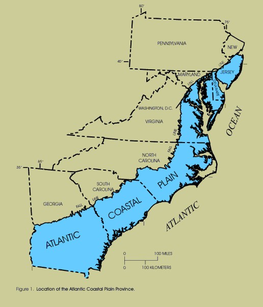 Figure 1. Location of the Atlantic Coastal Plain Province.
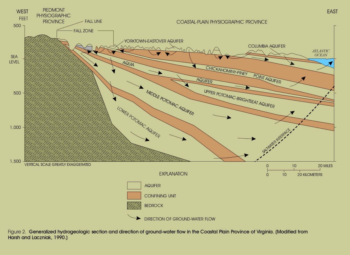 Figure 2. Generalized hydrogeologic section and direction of ground-water
flow in the Coastal Plain Province of Virginia. (Modified from Harsh and
Laczniak, 1990.)
Figure 2. Generalized hydrogeologic section and direction of ground-water
flow in the Coastal Plain Province of Virginia. (Modified from Harsh and
Laczniak, 1990.)
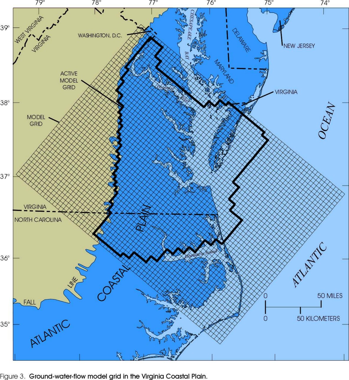 Figure 3. Grid of the ground-water-flow model of the Virginia Coastal Plain.
 Figure 4. Model transmissivity values representing the Columbia aquifer.
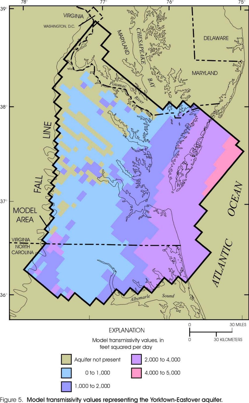 Figure 5. Model transmissivity values representing the Yorktown-Eastover
aquifer.
Figure 5. Model transmissivity values representing the Yorktown-Eastover
aquifer.
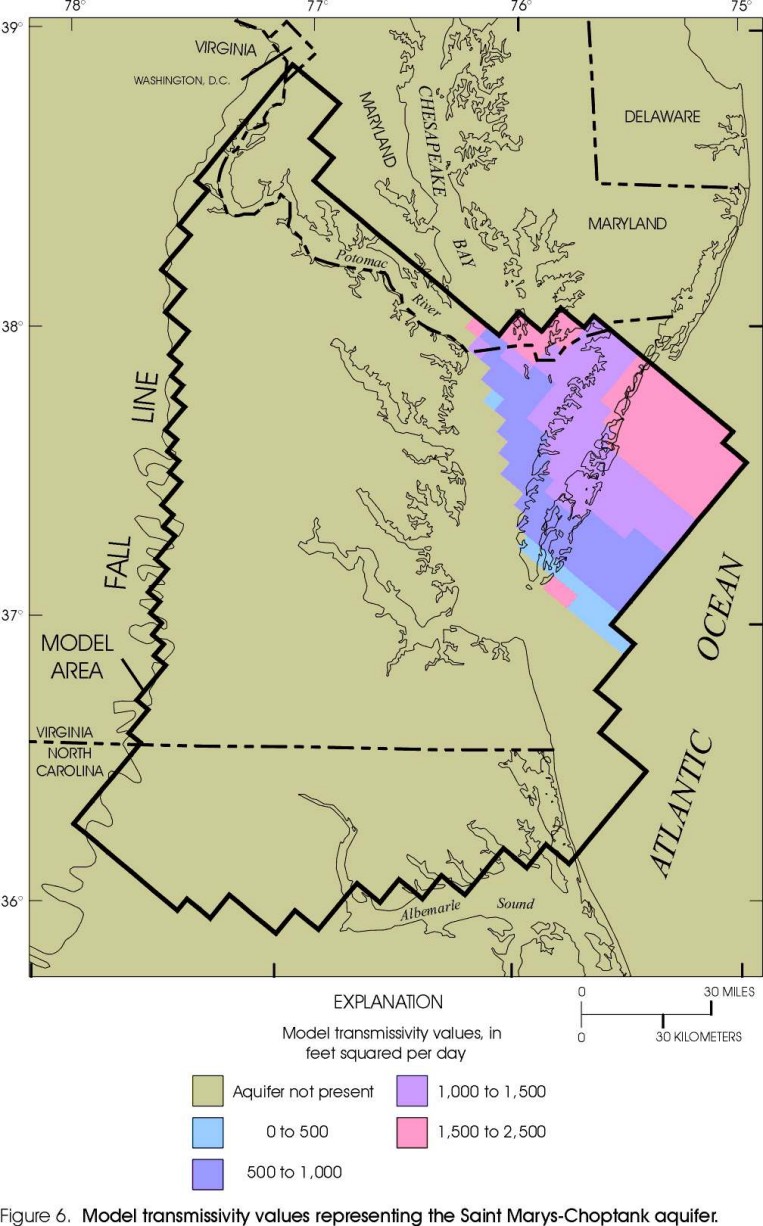 Figure 6. Model transmissivity values representing the Saint Marys-Choptank
aquifer.
Figure 6. Model transmissivity values representing the Saint Marys-Choptank
aquifer.
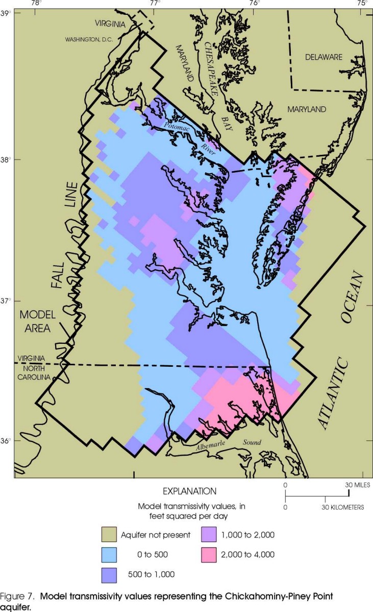 Figure 7. Model transmissivity values representing the Chickahominy-Piney
Point aquifer.
Figure 7. Model transmissivity values representing the Chickahominy-Piney
Point aquifer.
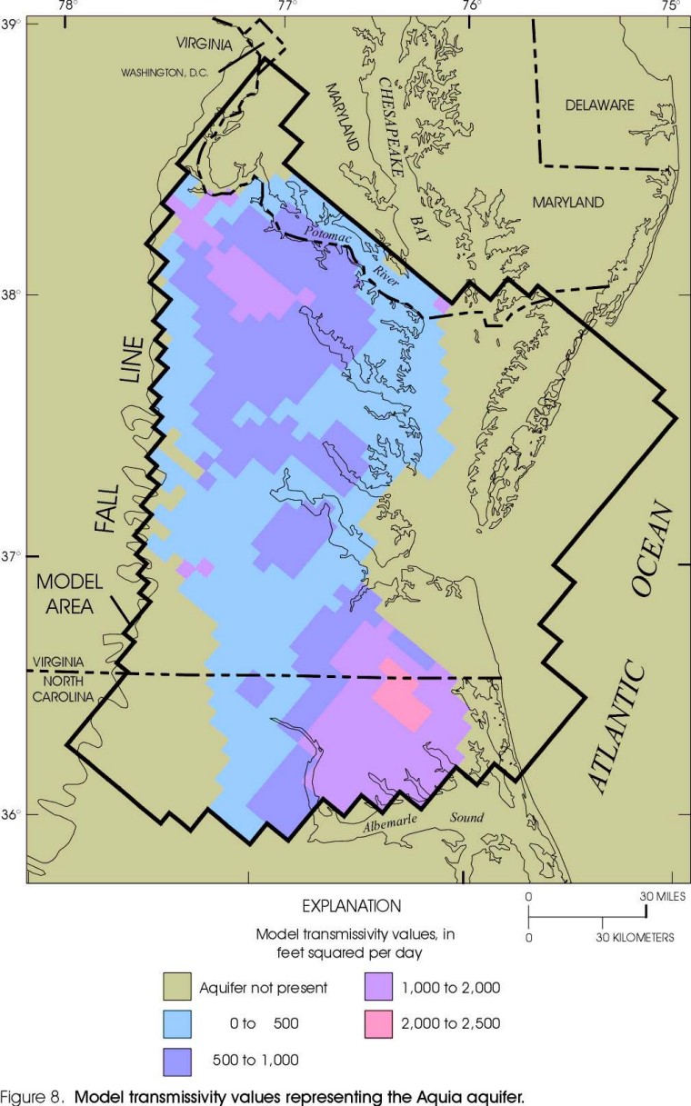 Figure 8. Model transmissivity values representing the Aquia aquifer.
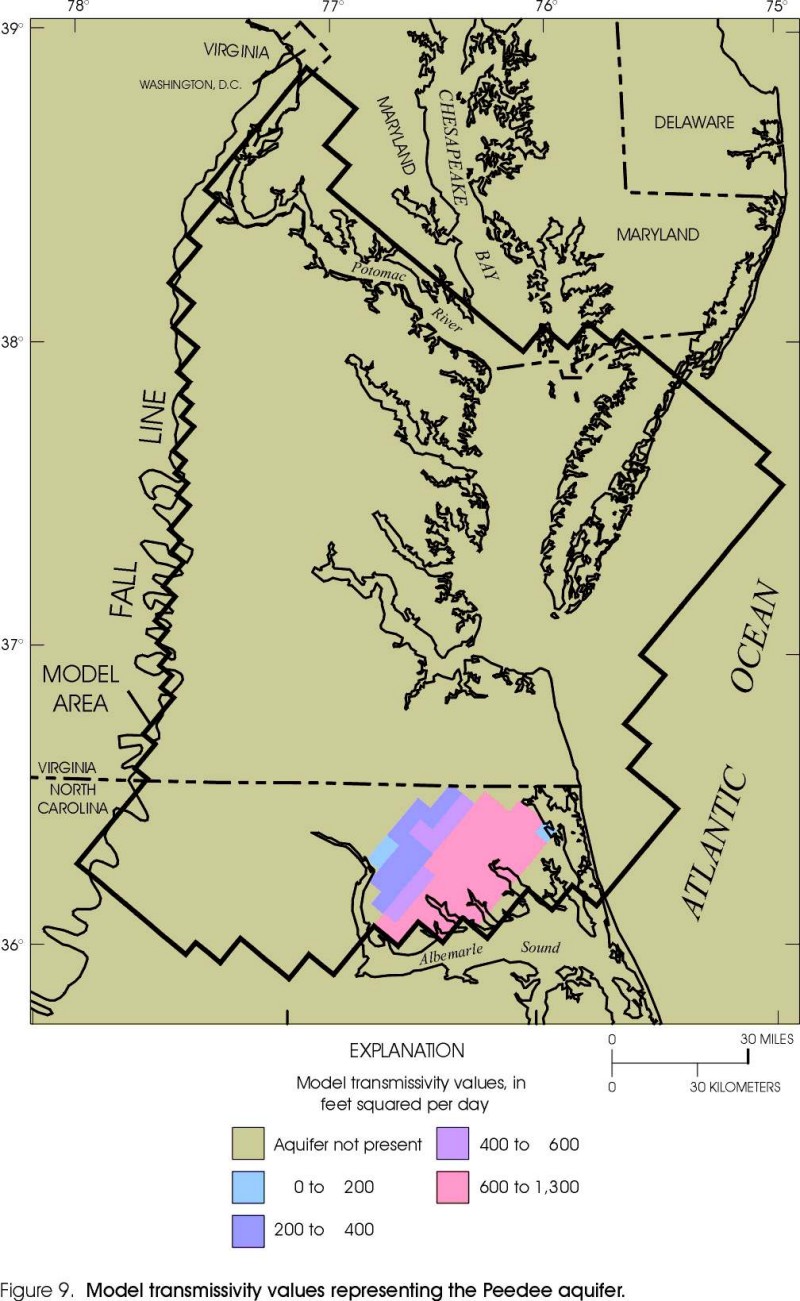 Figure 9. Model transmissivity values representing the Peedee aquifer.
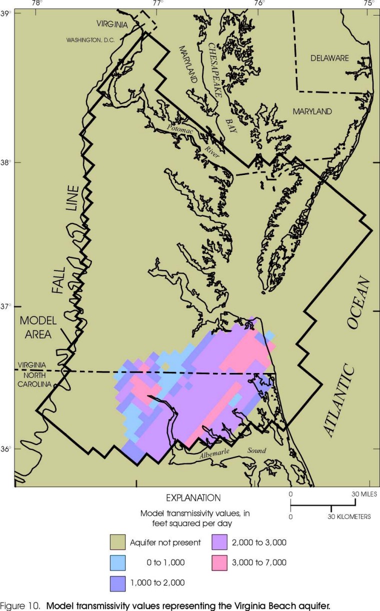 Figure 10. Model transmissivity values representing the Virginia Beach
aquifer.
Figure 10. Model transmissivity values representing the Virginia Beach
aquifer.
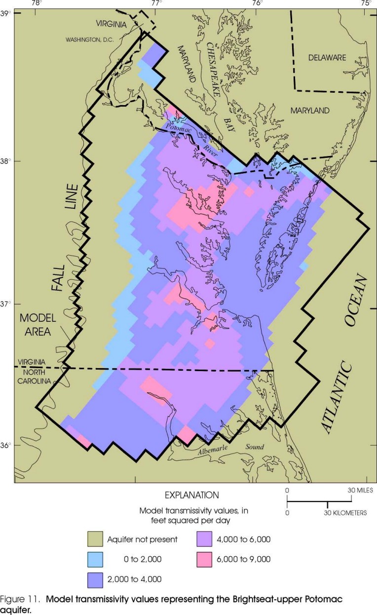 Figure 11. Model transmissivity values representing the Brightseat-upper
Potomac aquifer.
Figure 11. Model transmissivity values representing the Brightseat-upper
Potomac aquifer.
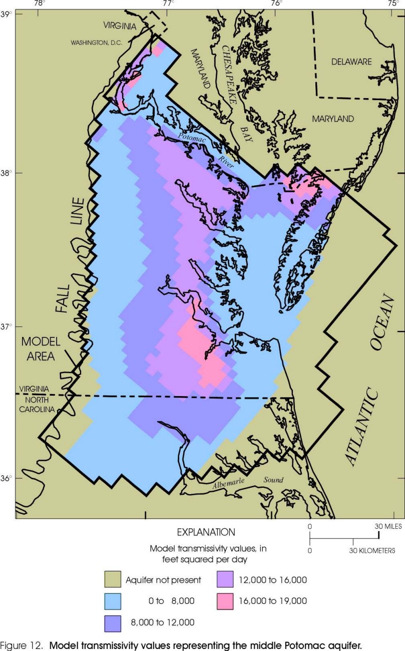 Figure 12. Model transmissivity values representing the middle Potomac
aquifer.
Figure 12. Model transmissivity values representing the middle Potomac
aquifer.
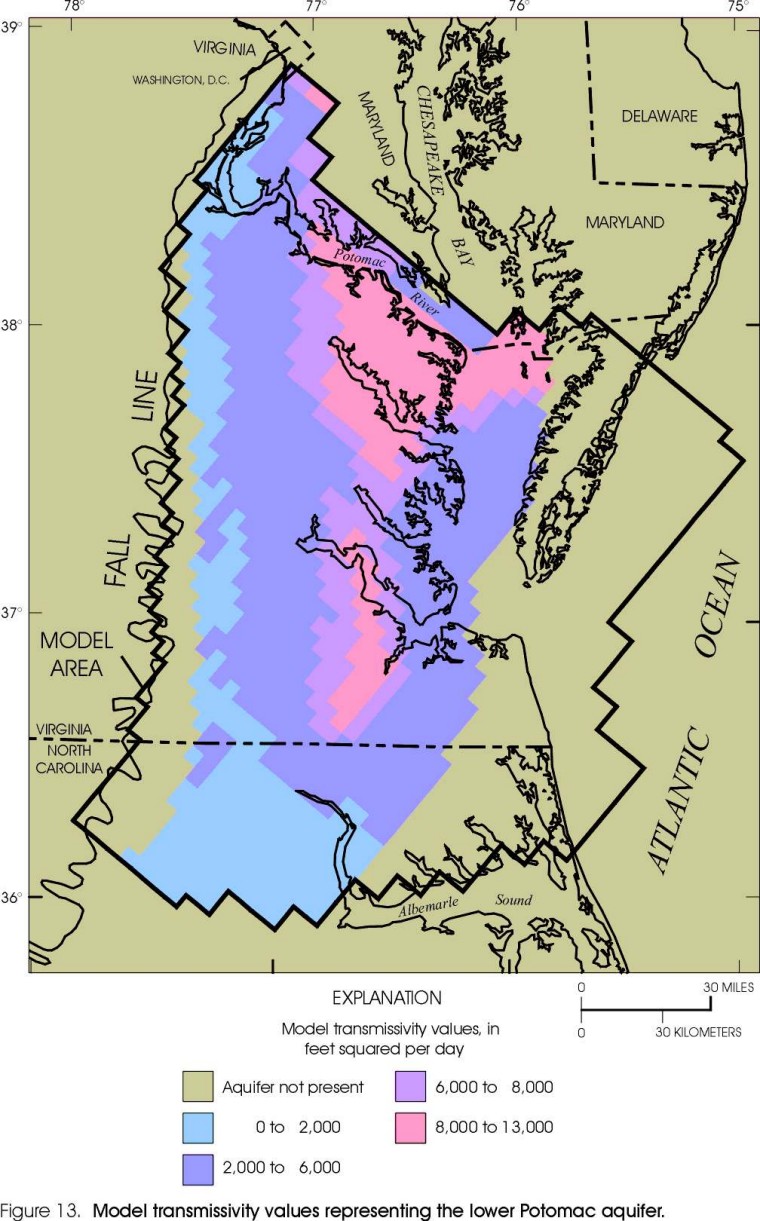 Figure 13. Model transmissivity values representing the lower Potomac aquifer.
 Figure 14. Model leakance values representing the Yorktown confining unit.
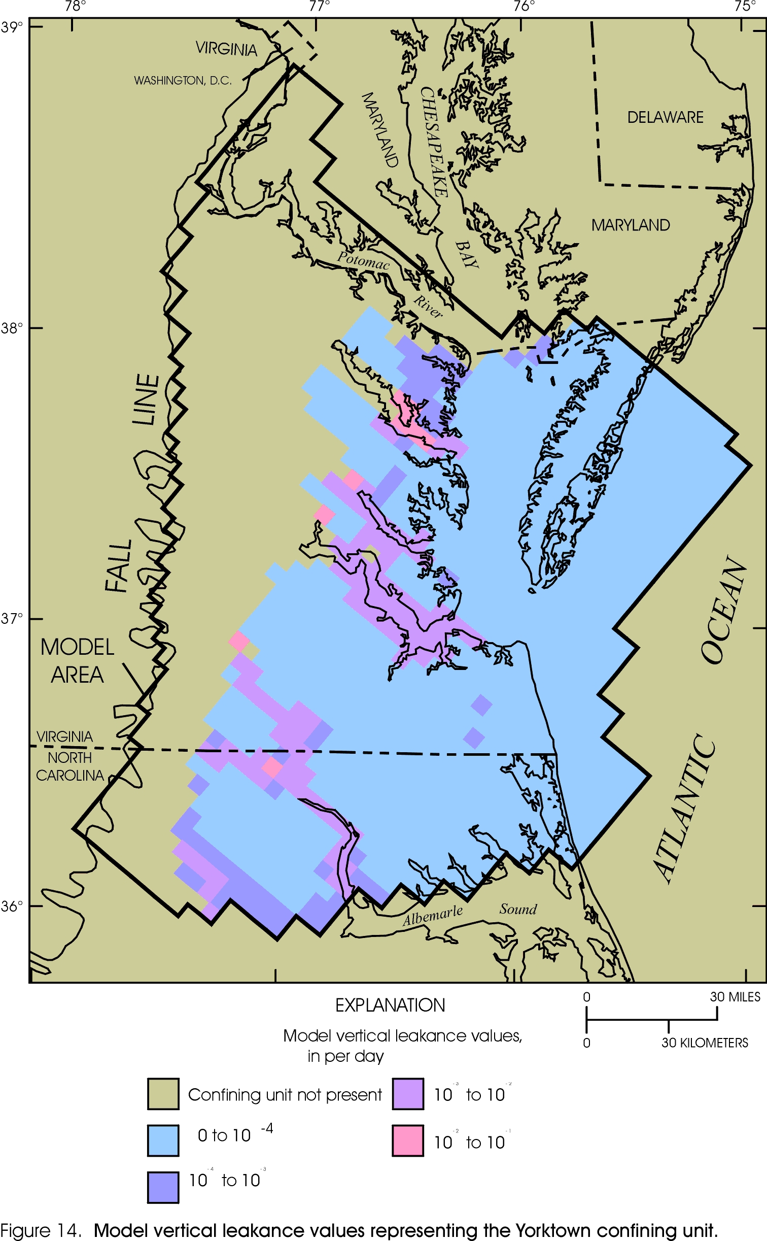 Figure 14.(test)
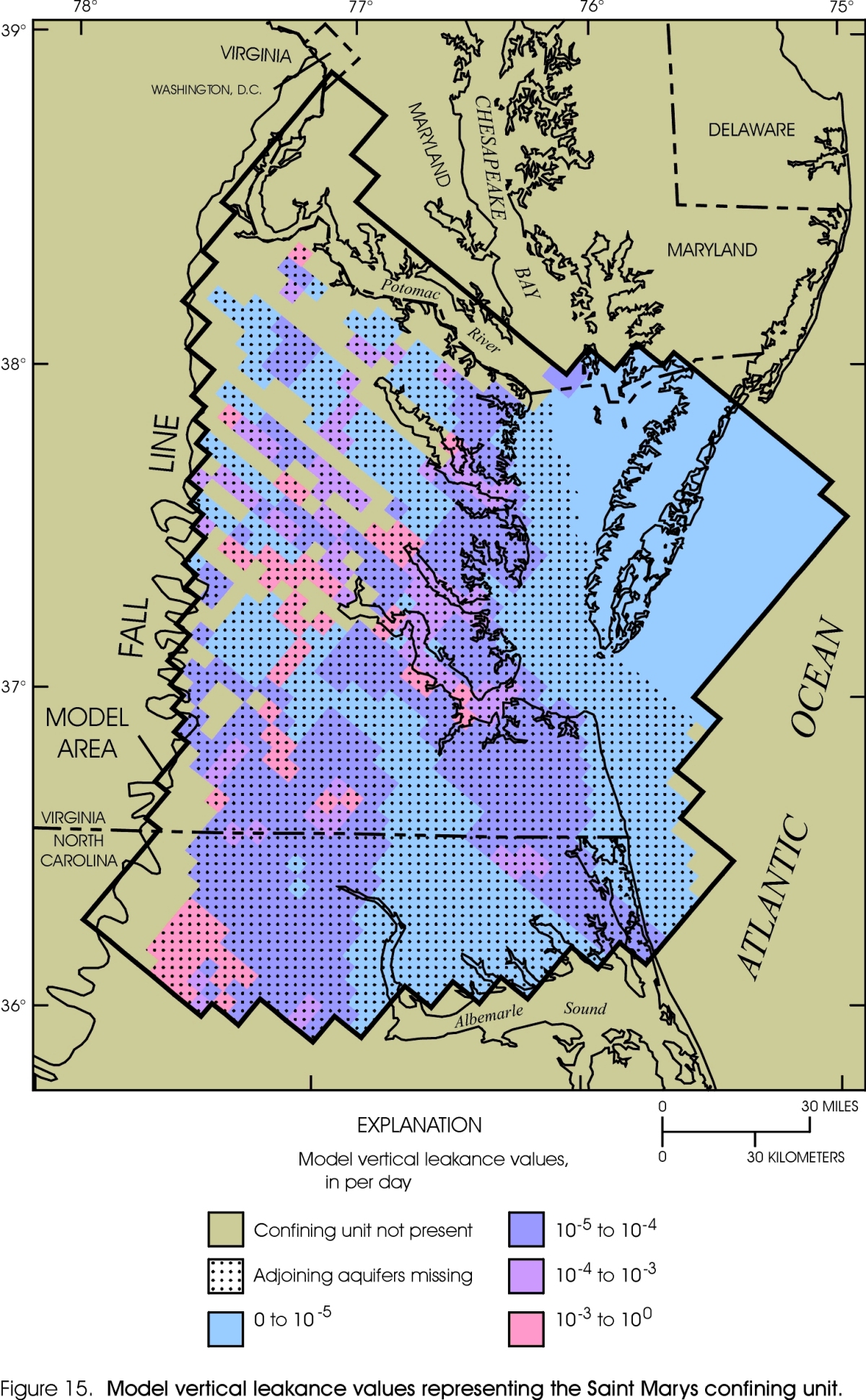 Figure 15. Model leakance values representing the Saint Marys confining
unit.
Figure 15. Model leakance values representing the Saint Marys confining
unit.
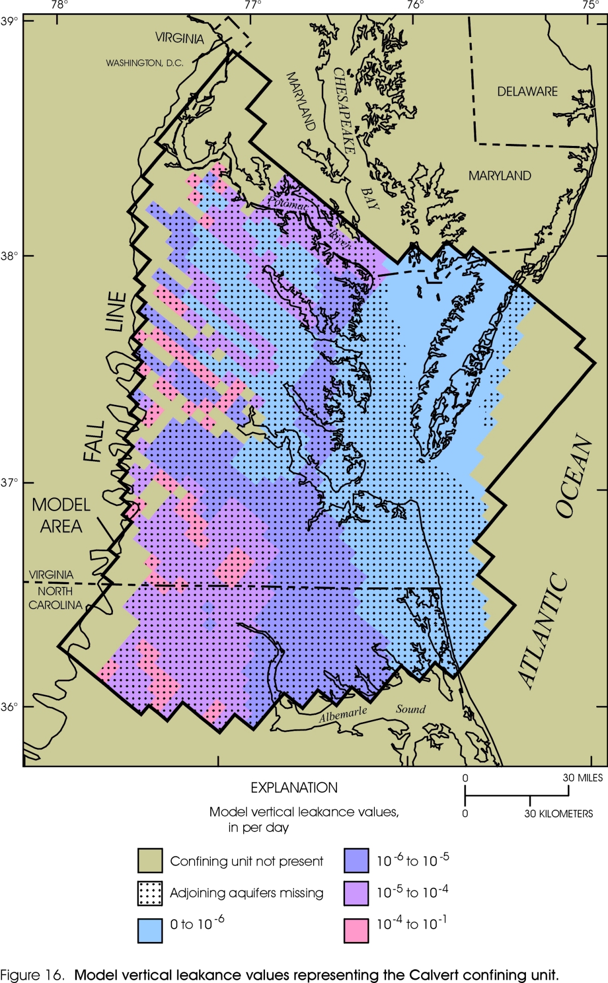 Figure 16. Model leakance values representing the Calvert confining unit.
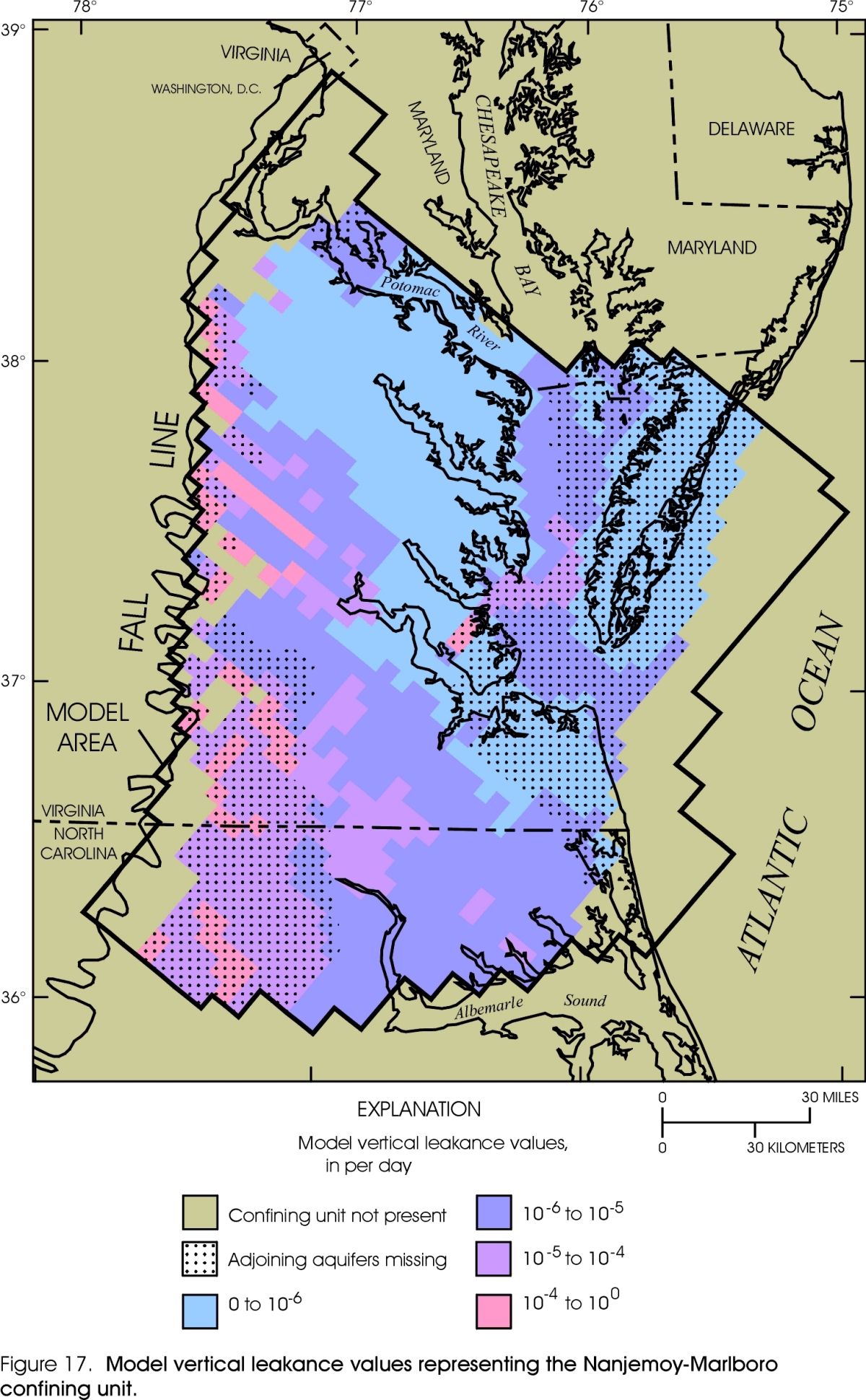 Figure 17. Model leakance values representing the Nanjemoy-Marlboro confining
unit.
Figure 17. Model leakance values representing the Nanjemoy-Marlboro confining
unit.
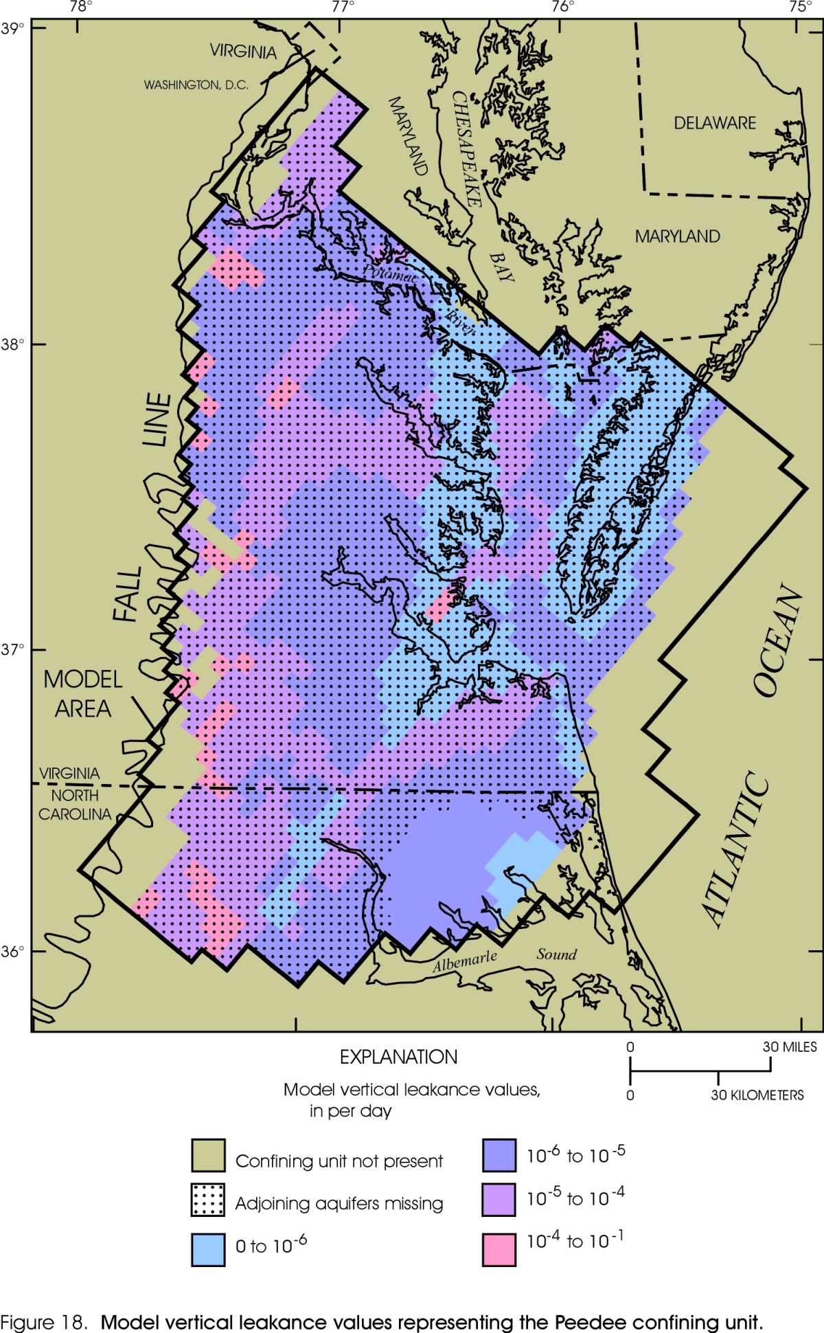 Figure 18. Model leakance values representing the Peedee confining unit.
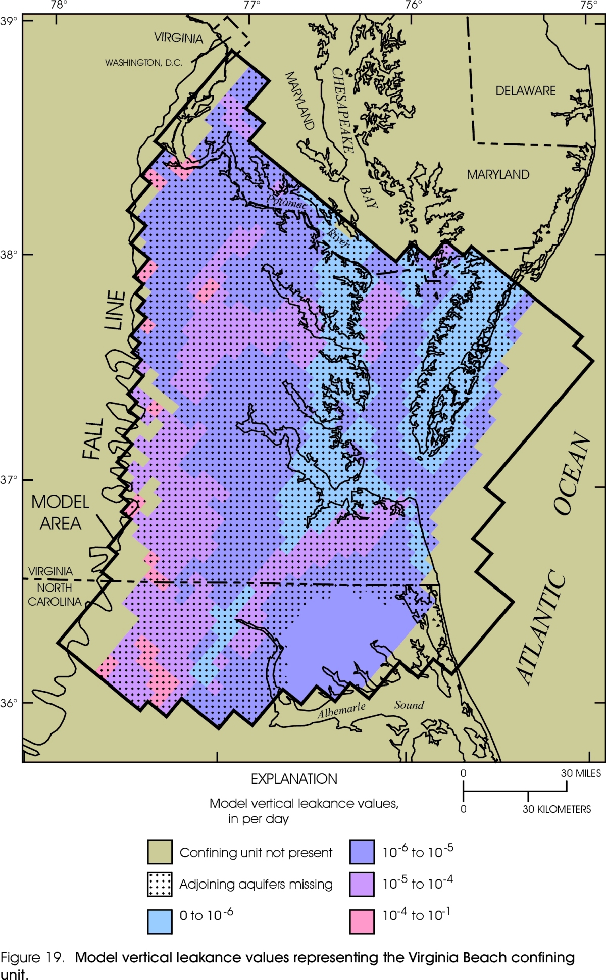 Figure 19. Model leakance values representing the Virginia Beach confining
unit.
Figure 19. Model leakance values representing the Virginia Beach confining
unit.
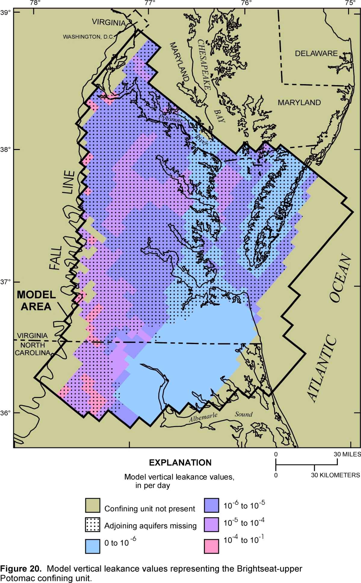 Figure 20. Model leakance values representing the Brightseat-upper Potomac
confining unit.
Figure 20. Model leakance values representing the Brightseat-upper Potomac
confining unit.
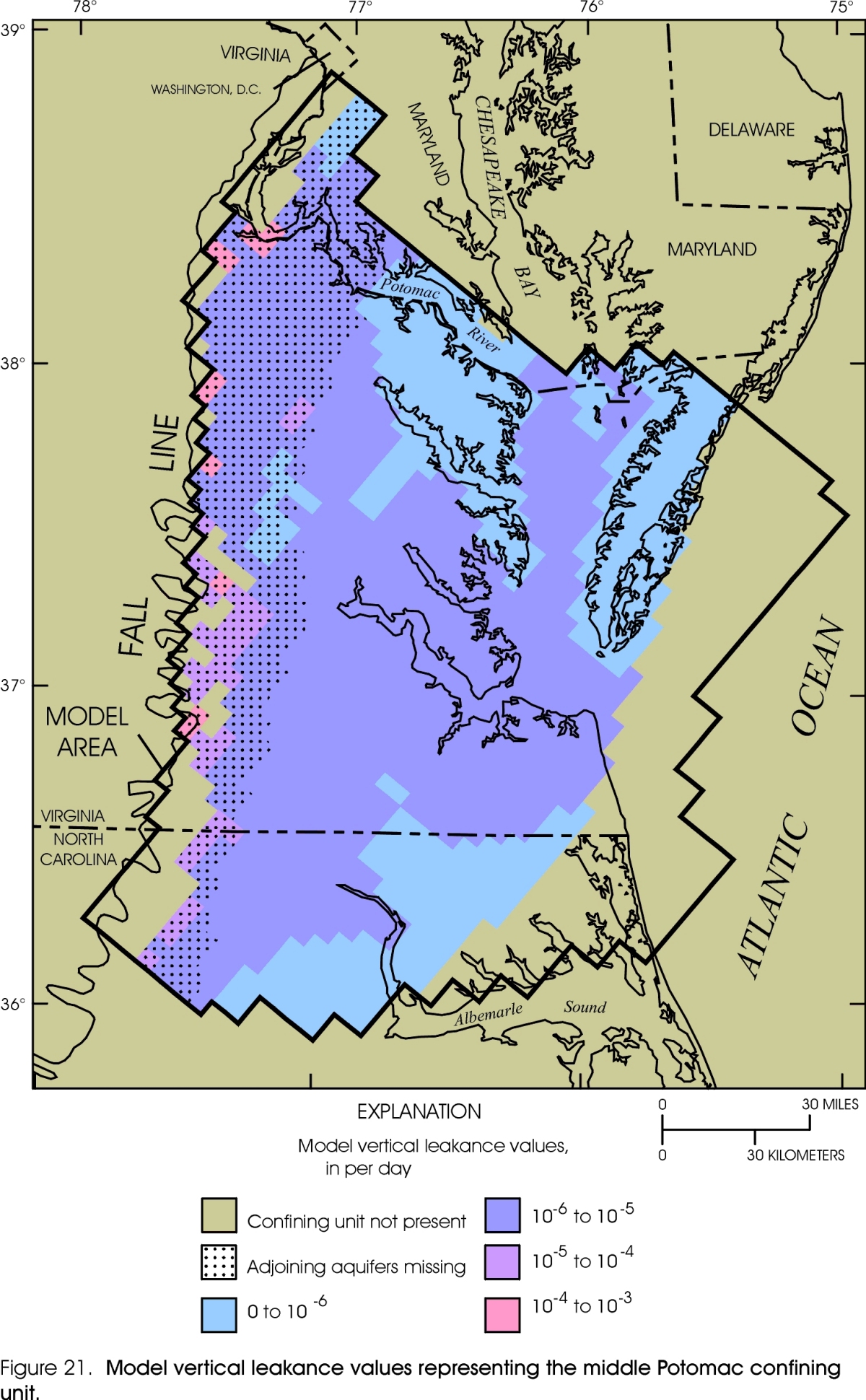 Figure 21. Model leakance values representing the middle Potomac confining
unit.
Figure 21. Model leakance values representing the middle Potomac confining
unit.
 Figure 22. Model leakance values representing the lower Potomac confining
unit.
Figure 22. Model leakance values representing the lower Potomac confining
unit.
 Figure 23. Simulated water levels for 1978-80 in the Columbia aquifer.
 Figure 24. Simulated water levels for 1978-80 in the Yorktown-Eastover
aquifer.
Figure 24. Simulated water levels for 1978-80 in the Yorktown-Eastover
aquifer.
 Figure 25. Simulated water levels for 1978-80 in the Saint Marys-Choptank
aquifer.
Figure 25. Simulated water levels for 1978-80 in the Saint Marys-Choptank
aquifer.
 Figure 26. Simulated water levels for 1978-80 in the Chickahominy-Piney
Point aquifer.
Figure 26. Simulated water levels for 1978-80 in the Chickahominy-Piney
Point aquifer.
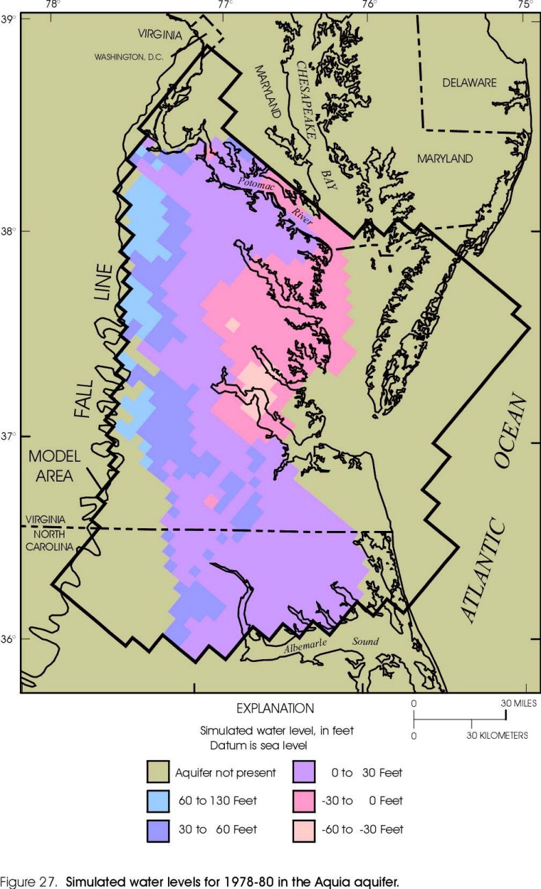 Figure 27. Simulated water levels for 1978-80 in the Aquia aquifer.
 Figure 28. Simulated water levels for 1978-80 in the Peedee aquifer.
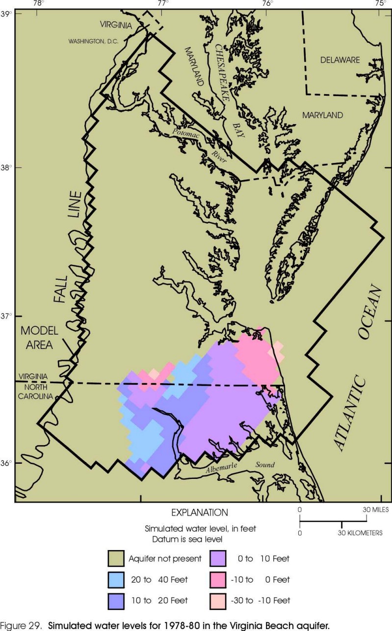 Figure 29. Simulated water levels for 1978-80 in the Virginia Beach aquifer.
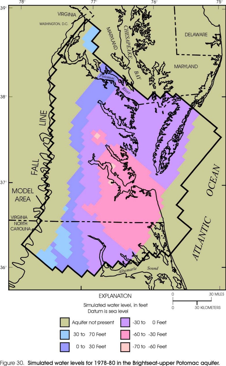 Figure 30. Simulated water levels for 1978-80 in the Brightseat-upper Potomac
aquifer.
Figure 30. Simulated water levels for 1978-80 in the Brightseat-upper Potomac
aquifer.
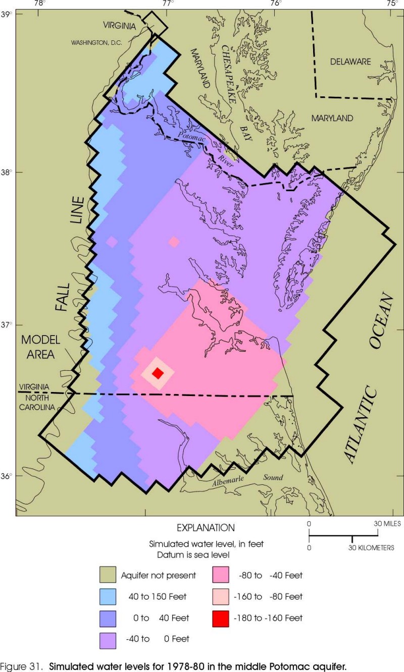 Figure 31. Simulated water levels for 1978-80 in the middle Potomac aquifer.
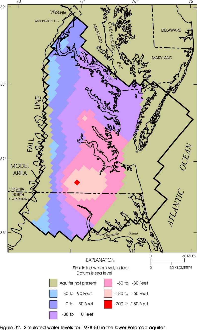 Figure 32. Simulated water levels for 1978-80 in the lower Potomac aquifer.